Table of Contents
- Why reuse someone else’s layers?
- How many layers should you reuse?
- The freeze, warm up, unfreeze routine
- Does it actually help? A small experiment
- What does the code look like?
- Gotchas worth knowing
- Sources and further reading
In this day and age it’s generally not a good idea to train a Deep Neural Network (DNN) from scratch without first checking whether an existing network already solves something close to your problem. Someone has probably spent far more compute, data and tuning effort on a similar task than you can afford to, and most of what their network learned is reusable. The practice of taking those learned layers and adapting them to a new task is known as Transfer Learning, and it buys you shorter training times, lower compute cost, and (most importantly) far better performance when your labelled data is limited.
This post covers the intuition for why reusing layers works, how to decide how much of a network to reuse, the standard freeze/unfreeze training routine, a small experiment demonstrating the payoff, and what the whole thing looks like in Keras.
Example: Imagine you need to classify images into a handful of custom categories. Instead of training a DNN from scratch, search for an existing model trained on a similar task (Hugging Face image classification models, Kaggle Models etc.)1, download it, and adapt it slightly to your task.
Why reuse someone else’s layers?
The reason this works at all comes down to what the different layers of a deep network learn. The lower layers (closest to the input) tend to learn generic, low-level features. In vision models that’s edges, textures and simple shapes; in language models, things like token co-occurrence patterns. The upper layers combine those into increasingly task-specific concepts, and the output layer is entirely specific to the original task and its exact set of labels.
Low-level features are useful for almost any task operating on the same kind of input. So if a network has already learned them from a large dataset, you can keep those layers as-is and only relearn the task-specific parts:
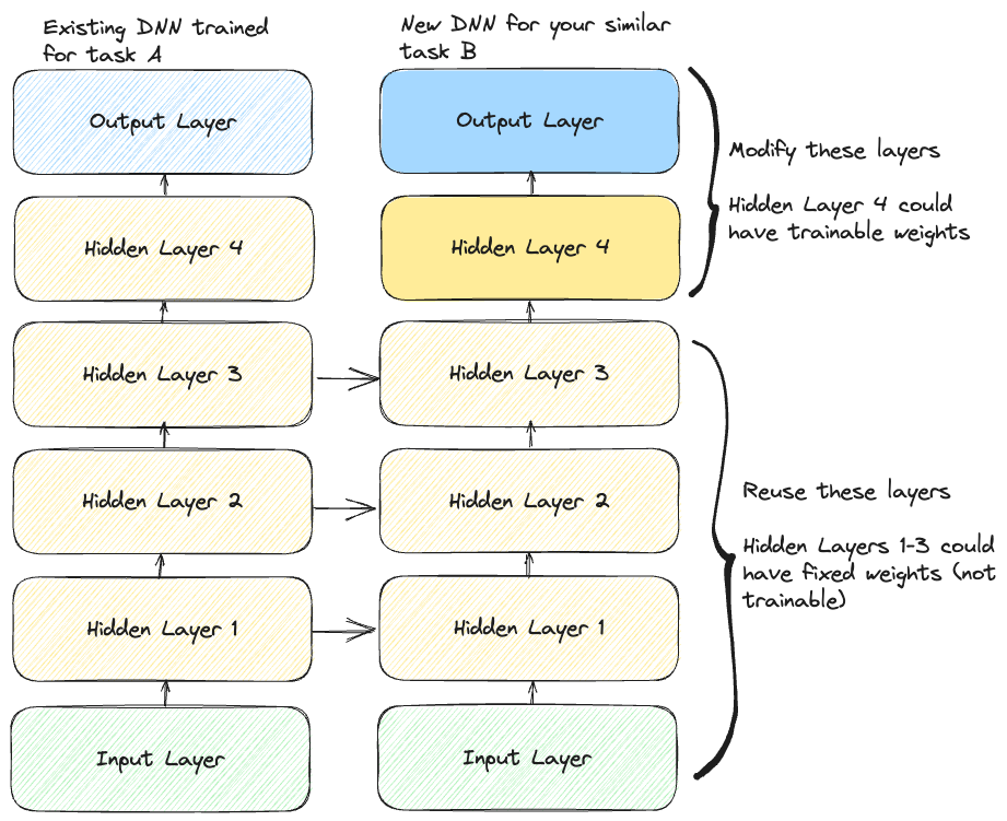
A few things follow directly from this picture:
- The output layer of the original model should almost always be replaced. The good pre-trained models tend to be foundational ones trained on large datasets with many classes, so their output layer is unlikely to match your label set. If you only want to distinguish 2 categories and the pre-trained model has 1000, that layer is useless to you.
- The upper hidden layers are less likely to be useful than the lower ones. High-level features are “overfit”, in a loose sense, to the original task. The closer a layer sits to the old output, the more task-specific its features are.
- Transfer works best when the inputs share low-level structure. Photos transfer to photos, audio spectrograms to audio spectrograms. If the input data doesn’t have the shape the original architecture expects, you’ll also need a preprocessing step to resize or reshape it.
How many layers should you reuse?
There’s no universal answer; it depends on two things: how similar the new task is to the original one, and how much labelled data you have for it.
The more similar the tasks, the more layers are worth keeping, starting from the bottom and working upwards. For very similar tasks you can often keep every hidden layer and only swap the output layer. The amount of data matters because every layer you unfreeze adds trainable parameters, and trainable parameters need data: with a small dataset you want most of the network frozen, while with a large one you can afford to re-train much more of it.

In practice, finding the right cut-off is an iterative process:
- Freeze all reused layers (make their weights non-trainable so gradient descent leaves them alone), train, and record the validation performance.
- Unfreeze the top one or two reused layers, train again, and see whether performance improves.
- Keep going while you’re seeing gains and have time to experiment. The more training data you have, the more layers you’ll find you can profitably unfreeze.
The freeze, warm up, unfreeze routine
There’s one subtlety that makes the freezing order matter. Your new output layer starts from random weights, so during the first few epochs it produces large, essentially random gradients. If the reused layers are trainable at that point, those gradients flow backwards and wreck the carefully pretrained weights before the head has settled down. The standard routine avoids this with two phases:

- Warm up the head. Freeze every reused layer, train for a few epochs, and let the new output layer learn sensible weights against stable, pretrained features.
- Fine-tune. Unfreeze some or all of the reused layers and keep training, but drop the learning rate substantially (a factor of 10 is a common starting point). The whole point of unfreezing is to make small refinements; a high learning rate at this stage will undo the transfer.
Does it actually help? A small experiment
To make the payoff concrete, I ran a small controlled experiment: a three-hidden-layer MLP implemented in plain numpy, on a synthetic dataset of 25 classes that all share the same underlying feature structure plus a heavy dose of nuisance variation (a stand-in for things like lighting and pose in real images). The source model is pretrained on 20 of the classes with plenty of data. The target task is to classify the 5 held-out classes from only a handful of examples, either by transferring the pretrained hidden layers (using the exact freeze-then-unfreeze routine above) or by training the same architecture from scratch. The full code is in the drop-down below if you want to poke at it.
The experiment code (click to expand)
import numpy as np

# ---- synthetic pair of related tasks ---------------------------------------
# Class identity lives in a 10-dim latent pushed through a fixed nonlinear map
# into 24 "signal" dims; 72 higher-variance structured "distractor" dims are
# stacked alongside (the stand-in for lighting/pose/background nuisance).
D_LATENT, D_STYLE = 10, 24      # class latent vs nuisance latent
D_SIGNAL, D_NOISE = 24, 72      # observed dims carrying signal vs distractors
D_HID_GEN = 48
D_X = D_SIGNAL + D_NOISE
N_CLASSES = 25
STYLE_SCALE = 2.5               # distractors have much higher variance

gen_rng = np.random.default_rng(0)
PROTOS = gen_rng.standard_normal((N_CLASSES, D_LATENT)) * 1.8
G1 = gen_rng.standard_normal((D_LATENT, D_HID_GEN)) / np.sqrt(D_LATENT)
G2 = gen_rng.standard_normal((D_HID_GEN, D_SIGNAL)) / np.sqrt(D_HID_GEN)
H = gen_rng.standard_normal((D_STYLE, D_NOISE)) / np.sqrt(D_STYLE)

def make_data(classes, n_per_class, rng):
    """Sample observations for the given classes through the shared map."""
    zs, ys = [], []
    for j, k in enumerate(classes):
        z = PROTOS[k] + 0.5 * rng.standard_normal((n_per_class, D_LATENT))
        zs.append(z)
        ys.append(np.full(n_per_class, j))
    z = np.vstack(zs)
    y = np.concatenate(ys)
    signal = np.tanh(np.tanh(z @ G1) @ G2)
    style = STYLE_SCALE * np.tanh(rng.standard_normal((len(z), D_STYLE)) @ H)
    x = np.hstack([signal, style]) + 0.05 * rng.standard_normal((len(z), D_X))
    p = rng.permutation(len(x))
    return x[p], y[p]

# ---- a tiny numpy MLP with Adam ---------------------------------------------
LAYERS = [D_X, 96, 48, 24]   # hidden stack; a softmax head sits on top

class MLP:
    def __init__(self, rng, n_out=5):
        dims = LAYERS + [n_out]
        self.W = [rng.standard_normal((a, b)) * np.sqrt(2.0 / a)
                  for a, b in zip(dims[:-1], dims[1:])]
        self.b = [np.zeros(b) for b in dims[1:]]
        self._adam = None

    def forward(self, x):
        acts = [x]
        for i, (W, b) in enumerate(zip(self.W, self.b)):
            x = x @ W + b
            if i < len(self.W) - 1:
                x = np.maximum(x, 0.0)
            acts.append(x)
        return acts

    def loss_grads(self, x, y):
        acts = self.forward(x)
        logits = acts[-1]
        logits = logits - logits.max(1, keepdims=True)
        p = np.exp(logits)
        p /= p.sum(1, keepdims=True)
        n = len(x)
        delta = p.copy()
        delta[np.arange(n), y] -= 1.0
        delta /= n
        gW, gb = [], []
        for i in range(len(self.W) - 1, -1, -1):
            gW.insert(0, acts[i].T @ delta)
            gb.insert(0, delta.sum(0))
            if i > 0:
                delta = (delta @ self.W[i].T) * (acts[i] > 0)
        return gW, gb

    def accuracy(self, x, y):
        return float((self.forward(x)[-1].argmax(1) == y).mean())

    def adam_step(self, gW, gb, lr, frozen_below=0,
                  beta1=0.9, beta2=0.999, eps=1e-8):
        if self._adam is None:
            self._adam = {
                "mW": [np.zeros_like(W) for W in self.W],
                "vW": [np.zeros_like(W) for W in self.W],
                "mb": [np.zeros_like(b) for b in self.b],
                "vb": [np.zeros_like(b) for b in self.b],
                "t": 0,
            }
        s = self._adam
        s["t"] += 1
        corr1 = 1 - beta1 ** s["t"]
        corr2 = 1 - beta2 ** s["t"]
        for i in range(len(self.W)):
            if i < frozen_below:      # frozen layers: no update
                continue
            for gs, ms, vs, ps in ((gW, s["mW"], s["vW"], self.W),
                                   (gb, s["mb"], s["vb"], self.b)):
                ms[i] = beta1 * ms[i] + (1 - beta1) * gs[i]
                vs[i] = beta2 * vs[i] + (1 - beta2) * gs[i] ** 2
                ps[i] -= lr * (ms[i] / corr1) / (np.sqrt(vs[i] / corr2) + eps)

def train(model, x, y, epochs, lr, rng, frozen_below=0, batch=32,
          x_val=None, y_val=None):
    """Minibatch training; returns per-epoch validation accuracy if given."""
    hist = []
    n = len(x)
    batch = min(batch, n)
    for _ in range(epochs):
        p = rng.permutation(n)
        for i in range(0, n, batch):
            idx = p[i:i + batch]
            gW, gb = model.loss_grads(x[idx], y[idx])
            model.adam_step(gW, gb, lr, frozen_below=frozen_below)
        if x_val is not None:
            hist.append(model.accuracy(x_val, y_val))
    return hist

# ---- the transfer protocol ----------------------------------------------------
SOURCE_CLASSES = list(range(20))     # broad source task -> generic features
TARGET_CLASSES = list(range(20, 25)) # five held-out classes, scarce data
WARMUP_EPOCHS, FINETUNE_EPOCHS = 40, 60
TOTAL_EPOCHS = WARMUP_EPOCHS + FINETUNE_EPOCHS
LR_BASE, LR_FINETUNE = 3e-3, 3e-4
N_HIDDEN_LAYERS = len(LAYERS) - 1

def pretrain_source(seed):
    rng = np.random.default_rng(1000 + seed)
    x, y = make_data(SOURCE_CLASSES, 800, rng)
    model = MLP(rng, n_out=len(SOURCE_CLASSES))
    train(model, x, y, epochs=50, lr=LR_BASE, rng=rng)
    return model

def run_target(seed, n_per_class, source_model, record_curves=False):
    """Train transfer and scratch models on the scarce target task."""
    rng = np.random.default_rng(2000 + seed)
    x_tr, y_tr = make_data(TARGET_CLASSES, n_per_class, rng)
    x_val, y_val = make_data(TARGET_CLASSES, 200, np.random.default_rng(99))

    # transfer: copy hidden layers, fresh head, warm up then fine-tune
    tr = MLP(rng)
    for i in range(N_HIDDEN_LAYERS):
        tr.W[i] = source_model.W[i].copy()
        tr.b[i] = source_model.b[i].copy()
    h1 = train(tr, x_tr, y_tr, WARMUP_EPOCHS, LR_BASE, rng,
               frozen_below=N_HIDDEN_LAYERS, x_val=x_val, y_val=y_val)
    h2 = train(tr, x_tr, y_tr, FINETUNE_EPOCHS, LR_FINETUNE, rng,
               x_val=x_val, y_val=y_val)

    # scratch: identical architecture and budget, random init
    sc = MLP(rng)
    h3 = train(sc, x_tr, y_tr, TOTAL_EPOCHS, LR_BASE, rng,
               x_val=x_val, y_val=y_val)

    if record_curves:
        return np.array(h1 + h2), np.array(h3)
    return tr.accuracy(x_val, y_val), sc.accuracy(x_val, y_val)

# ---- run everything -----------------------------------------------------------
SEEDS = range(10)
N_CURVE = 20                                   # per class, learning curves
N_SWEEP = [5, 10, 20, 50, 100, 250, 500]       # per class, data-size sweep

sources = {s: pretrain_source(s) for s in SEEDS}

curves_tr, curves_sc = zip(*(run_target(s, N_CURVE, sources[s],
                                        record_curves=True) for s in SEEDS))

for n in N_SWEEP:
    accs = [run_target(s, n, sources[s]) for s in SEEDS]
    tr_acc = np.mean([a[0] for a in accs])
    sc_acc = np.mean([a[1] for a in accs])
    print(f"n={n:>3}/class  transfer {tr_acc:.3f}  scratch {sc_acc:.3f}")

# plotting boilerplate omitted; the two panels are just means with
# one-standard-deviation bands over the 10 seeds

Three things stand out, and they generalise well beyond this toy setup:
- Transfer dominates when data is scarce. With 5 examples per class it nearly doubles the from-scratch accuracy (67% vs 35% here). The pretrained layers already know which directions of the input carry signal and which are noise, and that knowledge simply cannot be recovered from 25 examples.
- The unfreeze step earns its keep. The frozen-base model plateaus a few points below where fine-tuning ends up. Those upper-layer features were tuned to the source classes, and the low-learning-rate phase nudges them towards the new task.
- From scratch catches up when data is plentiful. Past a few hundred examples per class the two approaches converge, which is exactly why the quadrant chart above pushes you towards retraining more of the network as your dataset grows.
What does the code look like?
Below is what the workflow looks like in TensorFlow/Keras, assuming an existing original_model trained on a similar task and a new binary classification target:
import tensorflow as tf

# Load the pretrained model, then clone it so training doesn't
# quietly mutate the original weights (layers are shared objects,
# clone_model gives fresh copies)
original_model = tf.keras.models.load_model("original_model.keras")
base_model = tf.keras.models.clone_model(original_model)
base_model.set_weights(original_model.get_weights())

# New model: every layer except the old task-specific head,
# plus a fresh output layer for our binary task
new_model = tf.keras.Sequential(base_model.layers[:-1])
new_model.add(tf.keras.layers.Dense(1, activation="sigmoid"))

# Phase 1: freeze the reused layers so the randomly initialised
# head can't wreck the pretrained weights with its early gradients
for layer in new_model.layers[:-1]:
    layer.trainable = False

# Changing `trainable` only takes effect after a (re)compile
new_model.compile(loss="binary_crossentropy",
                  optimizer=tf.keras.optimizers.SGD(learning_rate=1e-3),
                  metrics=["accuracy"])
new_model.fit(X_train, y_train, epochs=5,
              validation_data=(X_valid, y_valid))

# Phase 2: unfreeze now that the head has warmed up
for layer in new_model.layers[:-1]:
    layer.trainable = True

# Recompile (mandatory after toggling trainable) with a much lower
# learning rate to protect the pretrained weights
new_model.compile(loss="binary_crossentropy",
                  optimizer=tf.keras.optimizers.SGD(learning_rate=1e-4),
                  metrics=["accuracy"])
new_model.fit(X_train, y_train, epochs=50,
              validation_data=(X_valid, y_valid))

new_model.evaluate(X_test, y_test)
You can imagine making this workflow more modular: wrap the freeze/train/unfreeze steps in a function parameterised by how many layers to reuse, and run the iterative search described earlier to find the best cut-off for your problem.
Note: The layer-slicing above assumes a
Sequentialmodel. For models built with the functional API you’d instead call the base model as a feature extractor and put new layers on top, as shown in the Keras transfer learning guide.
Gotchas worth knowing
- Match the original model’s preprocessing exactly. Pretrained weights assume inputs scaled, normalised and sized the way the original training data was. Most published models ship a preprocessing function; use it.
- Watch out for
BatchNormalizationlayers. They carry running statistics as well as weights. When you unfreeze them on a small, differently-distributed dataset, those statistics start updating and can destabilise training. Keeping batch norm layers frozen even in phase 2 is a common and sensible default. - Recompile after toggling
trainable. In Keras the change does nothing until the model is compiled again; forgetting this is a classic silent bug. - Depth matters. Transfer learning shines with deep networks (especially convolutional ones) because they’re the ones that learn a rich hierarchy of reusable features. With small, shallow dense networks there’s usually little worth transferring, a result explored systematically by Yosinski et al. (2014).
- Keep an honest baseline. If you have enough data to try it, also train from scratch. As the experiment above shows, transfer’s advantage shrinks as data grows, and it can even hurt slightly if the source task is a poor match (so-called negative transfer).
Sources and further reading
- Hands-On Machine Learning with Scikit-Learn, Keras & TensorFlow — Aurélien Géron’s chapter on training deep neural networks is the original basis for this post, including the freeze/unfreeze recipe.
- How transferable are features in deep neural networks? — Yosinski et al.’s NeurIPS 2014 paper quantifying the generic-to-specific transition across layers, the empirical backbone for “reuse lower layers first”.
- CS231n: Transfer Learning — Stanford’s course notes with practical rules of thumb along the same similarity-versus-data-size axes as the quadrant chart above.
- Keras: Transfer learning & fine-tuning — the canonical code companion, including the functional-API pattern and the batch norm caveat.
- Hugging Face Models and Kaggle Models — the two biggest catalogues for finding a pretrained starting point today.
-
There’s a chance you find a model that fits your task perfectly, so check several catalogues before settling on one. Papers with Code is also useful for finding the current best model for a task family. ↩